Lectures: Prof. Dr. Moritz Diehl, Exercises: Florian Messerer
*** Also see: Numerical Optimal Control (online). ***
The course’s aim is to give an introduction into numerical methods for the solution of optimization problems in science and engineering. The focus is on continuous nonlinear optimization in finite dimensions, covering both convex and nonconvex problems. It is intended for a mixed audience of students from mathematics, engineering and computer science.
The course is intended for self-study and is based on three pillars:
- a course manuscript
- lecture recordings, and
- exercises, that are accompanied with solutions and solution recordings.
Each of the three pillars is explained below. The recommended course duration is 12 weeks, with an overall workload of 10-20 hours per week. An example week of self-study could comprise e.g. 3 hours for reading the manuscript, 3 hours for watching two lectures, 4 hours for solving exercises.
Contact: moritz.diehl@imtek.uni-freiburg.de, florian.messerer@imtek.uni-freiburg.de
*** This page is intended as a timeless version of the course with a focus on self study of the material. For the most recent iteration of the course as taught for students of the university of Freiburg, see here. ***
Manuscript
The lectures are closely following a course manuscript draft. This manuscript is the first of three pillars for self-study.
Numerical optimization (draft manuscript) by M. Diehl
Lectures
The video recordings correspond each to approximately 90 minutes, and comprise 24 lectures in total. These recordings are the second pillar for self-study, and it is recommended to watch about two lectures per week.
| Lecture | Content |
| Lecture 1 | Introduction to Section 1.3 (Mathematical formulation) |
| Lecture 2 | Section 1.4 (Definitions) to 2.7 (Mixed-Integer-Programming) |
| Lecture 3 | Section 3.1 (How to check convexity) to 3.5 (Standard form of convex opt. problems) |
| Lecture 4 | Section 3.6 (Semidefinite Programming) to Example 4.2 (Dual of LP) |
| Lecture 5 | Example 4.3 (Dual decomposition) to Chapter 6 introduction |
| Lecture 6 | Section 6.1 (Linear Least Squares) to 6.5 (L1-Estimation) |
| Lecture 7 | Section 6.6 (Gauss-Newton method) to 7.2 (Local convergence rates) |
| Lecture 8 | Section 7.3 (Newton-Type methods) to 8.1 (Local contraction) |
| Lecture 9 | Section 8.2 (Affine invariance) to 9.1 (Line search) |
| Lecture 10 | Section 9.2 (Wolfe conditions) to 9.3 (Global convergence of line search) |
| Lecture 11 | Section 9.4 (Trust-Region methods) to 9.5 (The Cauchi-Point) |
| Lecture 12 | Section 10.1 (Algorithmic Differentiation) to 10.3 (Backward AD) |
| Lecture 13 | Section 10.4 to Chapter 11 introduction |
| Lecture 14 | Section 11.1 (LICQ and linearized feasible cone) to 11.2 (SONC) |
| Lecture 15 | Section 12.1 (Optimality conditions) to 12.5 (Constrained Gauss-Newton) |
| Lecture 16 | Section 11.3 (Perturbation analysis) and 12.7 (Local convergence) |
| Lecture 17 | Section 12.6 (General constrained NT-Algorithm) to 12.9 (Careful BFGS updating) |
| Lecture 18 | Section 13.1 to 13.2 (Active constraints and LICQ) |
| Lecture 19 | Section 13.3 (Convex Problems) |
| Lecture 20 | Section 13.4 (Complementarity) to 14.1 (QPs via Active Set Method) |
| Lecture 21 | Section 14.2 (SQP) to 14.4 (Interior Point methods) |
| Lecture 22 | Section 14.4 (Barrier problem interpretation, SCP) to 15.5 (Simultaneous optimal control) |
| Lecture 23 | Problem reformulations and useful function approximations |
| Lecture 24 | Summary of the course |
Exercises
The exercises are based partially on pen and paper and partially on (Matlab or Python) and CasADi (see below). They are the third pillar of the course, and it is recommended to do work on half an exercise sheet per week.
CasADi installation
CasADi is a symbolic framework for algorithmic differentiation and numerical optimization. In order to install CasADi, follow the instructions here. Download the binaries for your platform and, after having extracted them, add their location to Matlab's path. To test your installation run the simple example described at the provided link. If successful, save the path by executing the command savepath. In this way, the location of the binaries will be known even after restarting MATLAB.
Further Material
- Books
- Jorge Nocedal and Stephen J. Wright, Numerical Optimization, Springer, 2006
- Stephen Boyd and Lieven Vandenberghe, Convex Optimization, Cambridge Univ. Press, 2004
- Amir Beck, Introduction to Nonlinear Optimization, MOS-SIAM Optimization, 2014.
- simple midterm quiz
- sample exam
Winter semester 2020/21
The content below is only relevant for students who followed the course in the winter semester 2020/21.
Organization of the course
The course is organized as flipped classroom. We provide recordings of the lecture and will meet once a week to discuss the course contents. This course has 6 ECTS credits. It is possible to do a project to get an additional 3 ECTS, i.e., a total of 9 ECTS for course+project. For more information please contact Florian Messerer.
Virtual meetings: We will meet every Friday, 2.15pm to 4.00pm, in a virtual lecture room. These meetings are alternatingly dedicated to either Q&A sessions with Prof. Diehl or exercise sessions with the teaching assistant (see below). We will use Zoom for the meetings. Please note that you can join the meeting via your browser and do not need to install to the Zoom client. You can join via this link (Meeting ID: 858 1034 4638). The password is nUQtQw09? . Except for the kick-off session, none of the meetings will be recorded (edit: we decided to also not record the kick-off session, but you can find all relevant information on this page). For more information on how the university uses Zoom, a guide for students, and a note on data protection please see here.
Ilias: There is also an Ilias course, though most material will be published on the page you are currently viewing. In Ilias, we provide a forum for discussion of any questions you have related to the course, be it organization, content or exercises. Please feel free to open new topics and to answer questions of your fellow students. Further, the mid term quiz will be published on Ilias (see below). You can join the Ilias course via this link.
Lecture recordings: The lecture recordings were already created in a past semester. There are 24 lectures of approximately 90 minutes each. You can find the recordings below in the materials section, and a recommended schedule in the calendar.
Course manuscript: The lectures are accompanied by a detailed course manuscript, which you may find in the materials section below.
Exercises: The exercises are mainly computer based. Computers with MATLAB and CasADi installed are required to solve them (see below for details). The exercises are voluntary (though of course we strongly recommend to solve them). Nonetheless we offer the possibility to hand them in to receive feedback, but for this please respect the deadlines you can find in the calendar below. If you would like feedback on a specific part of the exercise especially, you can state so on your solution sheet. To hand them in, send them in an email to florian.messerer@imtek.de.
Q&A sessions: Every second week there will be a virtual Q&A session with Prof. Diehl, where you can ask any questions about the course content. The format is meant to be highly interactive and depends strongly on your participation. We would recommend that while watching the video lectures or reading the course script, you write down any questions that come to your mind, such that you have them readily available for the Q&A sessions.
Exercise sessions: Every other week we will meet for the exercise sessions. They will not be used to show the solutions, but to discuss any questions related to the exercises. These can either be questions about the current exercise sheet or questions about the solution to the last sheet. As the Q&A sessions, this format depends heavily on your participance.
Mid term quiz: Some time before christmas, we will publish a quiz on Ilias, with questions covering the course contents so far. It is obligatory that you pass this quiz until Dec 18, 11.59pm, but you have infinitely many trials for doing so and will receive instant feedback by auto-grading. The quiz will be online at least one week before the deadline. Note that the questions will not necessarily be representative of an exam.
Final evaluation: The final exam is a written exam. Only pen, paper, a calculator and two A4 sheets (i.e., 4 pages) of self-chosen content are allowed (handwritten). For students from the faculty of engineering and the B.Sc. Math, this exam is graded. Students from the M.Sc. Math need to pass the written exam in order to take the graded 11ECTS oral exam.
Projects: (more detail in a section below) The optional project (3 ECTS) consists in the formulation and implementation of a self-chosen optimization problem or numerical solution method, resulting in documented computer code, a project report, and a public presentation. Project work starts in the last third of the semester. For students from the faculty of engineering the project is graded independently from the 6ECTS lecture. For students from the B.Sc. Math, the grade for the lecture&project 9ECTS module is solely determined by the written exam. For students from the M.Sc. Math the project is again a prerequisite to the graded 11ECTS oral exam.
Calendar
| Date | Format | Content | watch this week | deadlines |
|---|---|---|---|---|
| Nov 06 | Intro | lec. 1, 2 | ||
| Nov 13 | Ex | ex1.pdf, ex1.zip | lec. 3, 4 | |
| Nov 20 | Q&A | up to chap 6.6 | lec. 5, 6 | ex1 (voluntary) |
| Nov 27 | Ex | ex2.pdf, ex1_sol, ex1_sol.zip | lec. 7, 8 | |
| Dec 04 | Q&A | up to chap 9.3 | lec. 9, 10 | ex2 (voluntary) |
| Dec 11 | Ex | lec. 11, 12 | ||
| Dec 18 | Q&A | up to chap 11.2 | lec. 13, 14 | ex3 (voluntary) / mid term quiz in illias (obligatory, until 11:59 pm) |
| *** | *** | *** Christmas *** | *** | *** |
| Jan 08 | Ex | ex4.pdf, ex4.zip, ex3_sol, ex3_sol.zip | lec. 15, 16 | |
| Jan 15 | Q&A | up to chap 13.2 | lec. 17, 18 | ex4 (voluntary) |
| Jan 22 | Ex | lec. 19, 20 | ||
| lec. 21, 22 | ex5 (voluntary) | |||
| Feb 05 | Ex | ex5_sol, ex5_sol.pdf | lec. 23, 24 | |
| Feb 12 | Q&A | all course content! |
Material
- lecture notes
- past exam
- PDF version of midterm quiz
Jorge Nocedal and Stephen J. Wright, Numerical Optimization, Springer, 2006.
Stephen Boyd and Lieven Vandenberghe, Convex Optimization, Cambridge Univ. Press, 2004.
Amir Beck, Introduction to Nonlinear Optimization, MOS-SIAM Optimization, 2014.
- Lecture recordings
| 1 | Part1 / Part2 | full* | Introduction to Section 1.3 (Mathematical formulation) | |
| 2 | Part1 / Part2 | full* | Section 1.4 (Definitions) to 2.7 (Mixed-Integer-Programming) | |
| 3 | Part1 / Part2 | full* | Section 3.1 (How to check convexity) to 3.5 (Standard form of convex opt. problems) | |
| 4 | Part1 / Part2 | full* | Section 3.6 (Semidefinite Programming) to Example 4.2 (Dual of LP) | |
| 5 | Part1 / Part2 | full* | Example 4.3 (Dual decomposition) to Chapter 6 introduction | |
| 6 | Part1 / Part2 | full* | Section 6.1 (Linear Least Squares) to 6.5 (L1-Estimation) | |
| 7 | Part1 / Part2 | full* | Section 6.6 (Gauss-Newton method) to 7.2 (Local convergence rates) | |
| 8 | Part1 / Part2 | full* | Section 7.3 (Newton-Type methods) to 8.1 (Local contraction) | |
| 9 | Part1 / Part2 | full* | Section 8.2 (Affine invariance) to 9.1 (Line search) | |
| 10 | Part1 / Part2 | full* | Section 9.2 (Wolfe conditions) to 9.3 (Global convergence of line search) | |
| 11 | Part1 / Part2 | full* | Section 9.4 (Trust-Region methods) to 9.5 (The Cauchi-Point) | |
| 12 | Part1 / Part2 | full* | Section 10.1 (Algorithmic Differentiation) to 10.3 (Backward AD) | |
| 13 | Part1 / Part2 | full* | Section 10.4 to Chapter 11 introduction | |
| 14 | Part1 / Part2 | full* | Section 11.1 (LICQ and linearized feasible cone) to 11.2 (SONC) | |
| 15 | Part1 / Part2 | full* | Section 12.1 (Optimality conditions) to 12.5 (Constrained Gauss-Newton) | |
| 16 | Part1 / Part2 | full* | Section 11.3 (Perturbation analysis) and 12.7 (Local convergence) | |
| 17 | Part1 / Part2 | full* | Section 12.6 (General constrained NT-Algorithm) to 12.9 (Careful BFGS updating) | |
| 18 | Part1 / Part2 | full* | Section 13.1 to 13.2 (Active constraints and LICQ) | |
| 19 | Part1 / - | full* | Section 13.3 (Convex Problems) | |
| 20 | Part1 / Part2 | full* | Section 13.4 (Complementarity) to 14.1 (QPs via Active Set Method) | |
| 21 | Part1 / Part2 | full* | Section 14.2 (SQP) to 14.4 (Interior Point methods) | |
| 22 | Part1 / Part2 | full* | Section 14.4 (Barrier problem interpretation, SCP) to 15.5 (Simultaneous optimal control) | |
| 23 | Part1 / Part2 | full* | Problem reformulations and useful function approximations | |
| 24 | Part1 / Part2 | full* | Summary of the course |
* Experimental: Both lecture parts merged and file size compressed. Please let us know if you experience any problems.
Project
For a more detailed description of the projects and their requirements, please see these guidelines.
There is a time slot separate from the normal sessions for discussing the projects. Starting on Jan 21st, we will meet each Thursday, 10am-12pm. At that point, you need to have sent your project idea via email (see guidelines), and registered for the SL/PL as required by your examination office (deadline depending on your examination office). The first session will be used to finalize your project ideas, and the following sessions to discuss your progress and the problems you face. The final presentations will be on March 08, and the deadline for the written project is March 18, 23:59.
| Date | Time | Content |
|---|---|---|
| Jan 21 | 10 - 12 | deadline project ideas, first project session |
| Jan 28 | 10 - 12 | project session |
| Feb 04 | 10 - 12 | project session |
| Feb 11 | 10 - 12 | project session |
| Feb 25 | 10 - 12 | project session |
| Mar 08 | 9:30 - 12:00 | project presentations (schedule below) |
| Mar 18 | 23:59 | project report deadline |
Project presentation schedule (March 08)
Time per talk: max 8 min (strict!) +2 min questions
| Time | Content |
| 09:30 - 09:35 | Welcome |
| 09:35 - 09:45 | Presentation 1 |
| 09:45 - 09:55 | Presentation 2 |
| 09:55 - 10:05 | Presentation 3 |
| 10:05 - 10:15 | Presentation 4 |
| 10:15 - 10:25 | Presentation 5 |
| 10:25 - 11:00 | Break |
| 11:00 - 11:10 | Presentation 6 |
| 11:10 - 11:20 | Presentation 7 |
| 11:20 - 11:30 | Presentation 8 |
| 11:30 - 11:40 | Presentation 9 |
| 11:40 - 11:45 | Concluding remarks |
Matlab and CasADi installation
MATLAB is an environment for numerical computing based on a proprietary language that allows one to easily manipulate matrices and visualize data which will be very helpful in prototyping the algorithms presented during the lectures of this course. The University of Freiburg offers a free-of-cost license to students and staff which can be obtained following the instructions here. In order to be able to complete the exercises of this course, you will need a working installation of MATLAB. Follow the instructions at the provided link in order to install the software package.
CasADi is a symbolic framework for algorithmic differentiation and numerical optimization. In order to install CasADi, follow the instructions here. Download the binaries for your platform and, after having extracted them, add their location to MATLAB's path. To test your installation run the simple example described at the provided link. If successful, save the path by executing the command savepath. In this way, the location of the binaries will be known even after restarting MATLAB.
Supplementary Links and Material for the Q&A Sessions
Mainly meant as reference for those who attended the respective session. Do not worry if you were not there and find the following content confusing.
- Q&A 1 (6.11.20)
- Optimal Throw Angle Team Question for Zoom Breakout Sessions: You are standing on top of a 10m high building and want to throw a tennis ball as far as possible, i.e., maximize the distance from the foot of the building to the touch-down point of the ball on the (horizontal) ground. The throwing velocity you can achieve is maximally 20m/s at the moment when the ball leaves your hand. At which angle should you throw the ball, i.e., what angle (in degrees) does the initial direction make with the horizontal? Please fill in your answer after a discussion of 5-10 minutes into the following google sheet together with optional supplementary information. This sheet will be shared among all course participants but taken off from the web after the session (link is removed).
- picture of black board with the problem formulated as Nonlinear Program (NLP)
- matlab code solving the NLP with CasADi -> Optimal angle is 39.32 degree.
- Note: Using numerical methods here might be seen as overkill, as this problem can probably also be easily solved analytically (as some of you did during the Q&A). But in general acquiring solutions analytically is intractable.
- Optimal Throw Angle Team Question for Zoom Breakout Sessions: You are standing on top of a 10m high building and want to throw a tennis ball as far as possible, i.e., maximize the distance from the foot of the building to the touch-down point of the ball on the (horizontal) ground. The throwing velocity you can achieve is maximally 20m/s at the moment when the ball leaves your hand. At which angle should you throw the ball, i.e., what angle (in degrees) does the initial direction make with the horizontal? Please fill in your answer after a discussion of 5-10 minutes into the following google sheet together with optional supplementary information. This sheet will be shared among all course participants but taken off from the web after the session (link is removed).
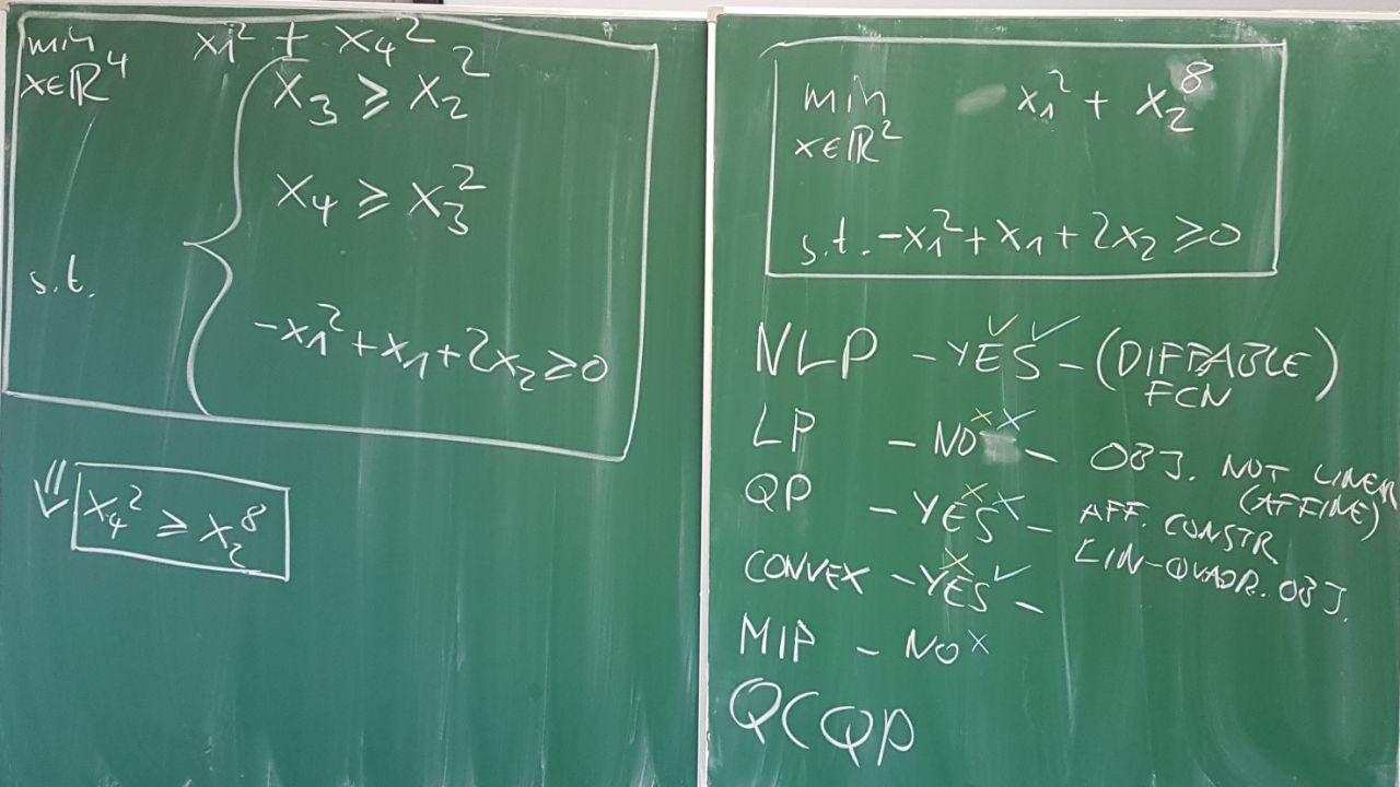
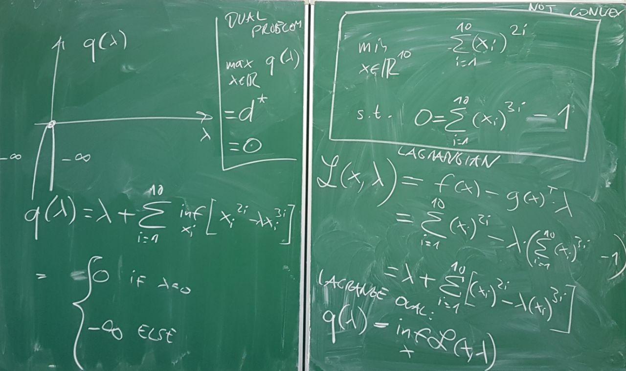
- Q&A 2 (20.11.20)
- Blackboard pictures:
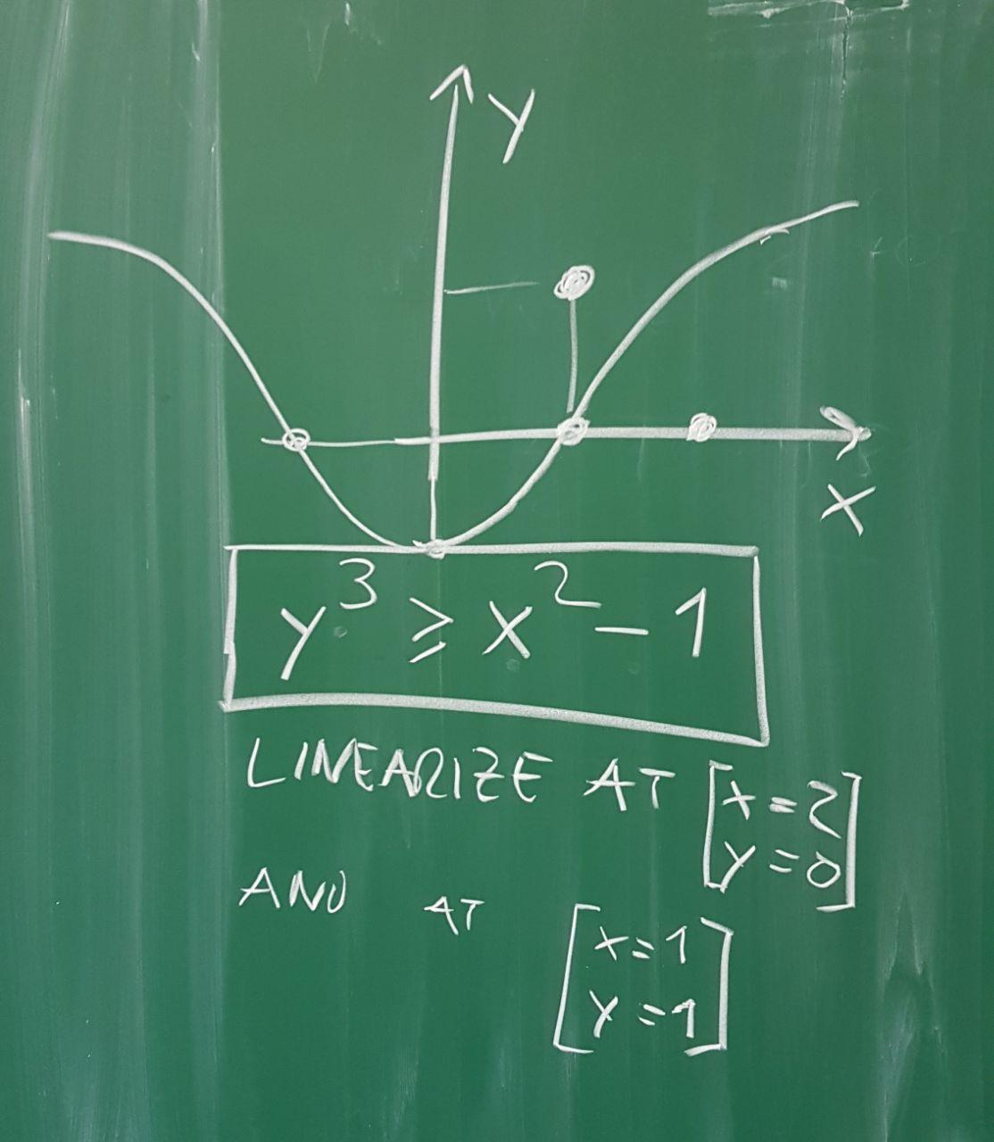
- Team Question: constraint linearization
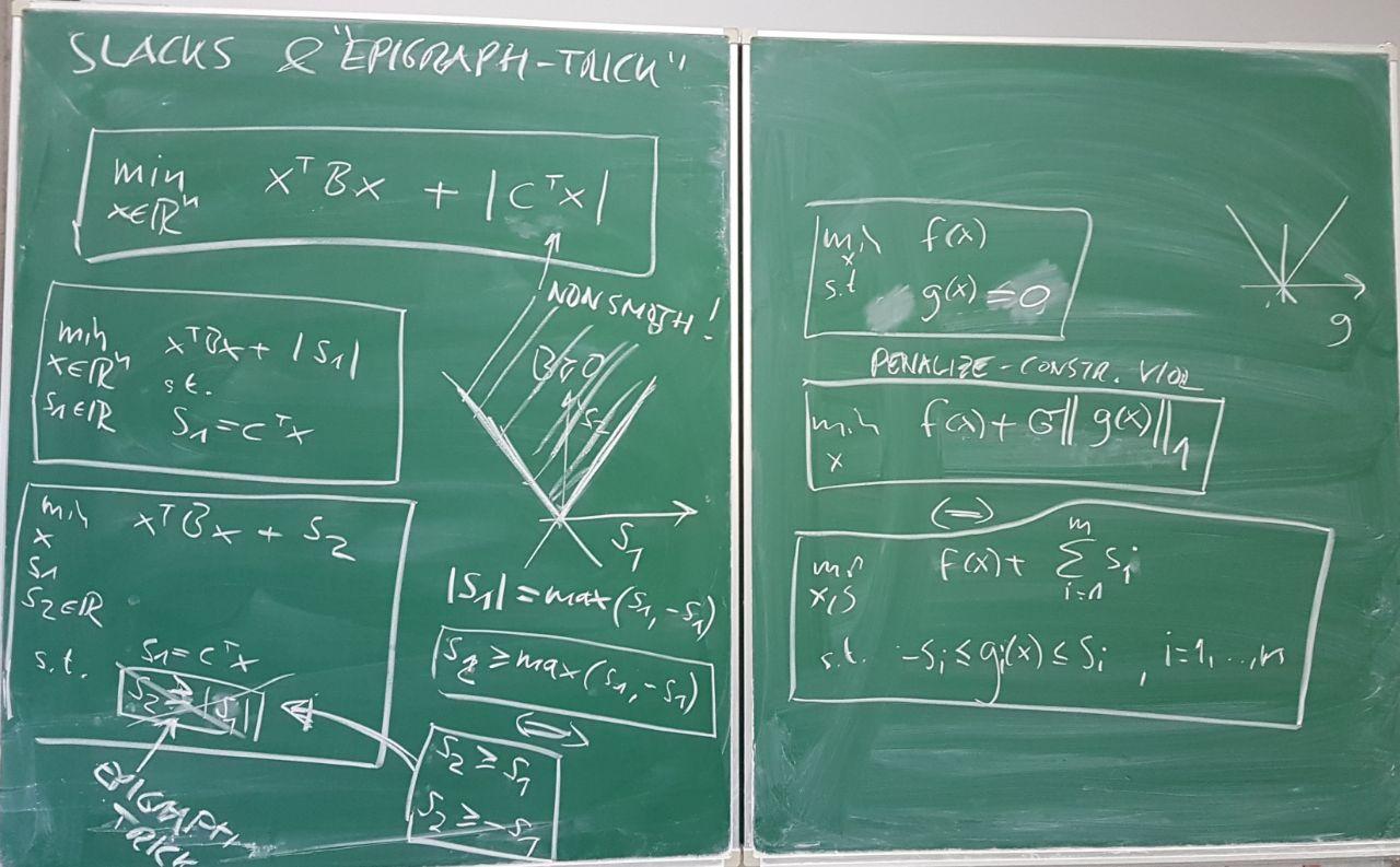
- Q&A 3 (4.12.20)
- Blackboard picture