Lectures: Prof. Dr. Moritz Diehl, Exercises: Florian Messerer
The course’s aim is to give an introduction into numerical methods for the solution of optimal control problems in science and engineering. The focus is on both discrete time and continuous time optimal control in continuous state spaces. It is intended for a mixed audience of students from mathematics, engineering and computer science.
*** This page is intended for the course as taught in the summer semester 2021 at the University of Freiburg. For a timeless version with a focus on self study of the material see here. ***
Contact: moritz.diehl@imtek.uni-freiburg.de, florian.messerer@imtek.uni-freiburg.de
Announcements
- The winter semester exam is on March 18, 9am. Writing time: 2h. Room: SR 02-016/18, G.-Köhler-Allee 101, Faculty of Engineering. See 'Final Evaluation' below for more detail.
Structure of the course
This course is organized as inverted classroom and we provide recordings of the lecture and of the exercise solutions. We will meet once a week to discuss lecture or exercises. The course has 6 ECTS credits. It is possible to do a project to get an additional 3 ECTS, i.e., a total of 9 ECTS for course+project.
Virtual meetings: We will meet every Friday at 10 a.m. sharp in a virtual lecture room. These meetings are alternatingly dedicated to either Q&A sessions with Prof. Diehl or exercise sessions with the teaching assistant (see below). We will use Zoom for the meetings. Please note that you can join the meeting via your browser and do not need to install to the Zoom client. Except for the kick-off session, none of the meetings will be recorded. For more information on how the university uses Zoom, a guide for students, and a note on data protection please see here.
https://uni-freiburg.zoom.us/j/64814305986
Meeting ID: 648 1430 5986
Passcode: nocse2021
Ilias: There is also an Ilias course, though most material will be published on the page you are currently viewing. In Ilias, we provide a forum for discussion of any questions you have related to the course, be it organization, content or exercises. Please feel free to open new topics and to answer questions of your fellow students. Further, the mid term quiz will be published on Ilias (see below).
Lecture recordings: The lecture recordings were already created in a past semester. There are 20 lectures of approximately 90 minutes each, which amounts to a lecture load of about 2 lectures or 3 hours per week. You can find a recommended schedule for watching them in the calender below.
Course manuscript: The lectures are accompanied by a detailed course manuscript, which you may find in the materials section below. Please note that it is in general more detailed than the lectures and that we skip some of the chapters.
Exercises: The exercises are mainly computer based. Computers with MATLAB and CasADi installed are required to solve them (see below for details). There will be a total of 10 exercises. They will be published throughout the semester, after some time delay followed by a solution manuscript as well as a video recording. The exercises are voluntary (though of course we strongly recommend to solve them). Nonetheless we offer the possibility to hand them in to receive feedback, but for this please respect the deadlines you can find in the calendar below. If you would like feedback on a specific part of the exercise especially, you can state so on your solution sheet.
Q&A sessions: Every second week there will be a virtual Q&A session with Prof. Diehl, where you can ask any questions about the course content. The format is meant to be highly interactive and depends strongly on your participation. We would recommend that while watching the video lectures or reading the course script, you write down any questions that come to your mind, such that you have them readily available for the Q&A sessions.
Exercise sessions: Every other week we will meet for the exercise sessions. They will not be used to show the solutions, but to discuss any questions related to the exercises. These can either be questions about the current exercise sheet or questions about the solution to the last sheet. As the Q&A sessions, this format depends heavily on your participance.
Mid term quiz: Some time during the semester, we will publish a quiz on Ilias, with questions covering the course contents so far. It is obligatory that you pass this quiz until a deadline (to be specified), but you have infinitely many trials and at least one week for doing so and will receive instant feedback by auto-grading. Note that the questions will not necessarily be representative of an exam.
Final evaluation: The final exam is a written closed book exam. Only pen, paper, a calculator and two A4 sheets (i.e., 4 pages) of self-chosen content are allowed (handwritten). Everyone who wants ECTS for this course needs to pass the exam. For students from the faculty of engineering and the B.Sc. Math, this exam is graded. Students from the M.Sc. Math need to pass the written exam in order to take a graded 11ECTS oral exam.
Projects (more detail in a section below): The optional project (3 ECTS) consists in the formulation and implementation of a self-chosen problem of Numerical Optimal Control, resulting in documented computer code, a project report, and a public presentation. Project work starts in the last third of the semester. For students from the faculty of engineering the project is graded independently from the 6ECTS lecture. For students from the B.Sc. Math, the grade for the lecture&project 9ECTS module is solely determined by the written exam. For students from the M.Sc. Math the project is again a prerequisite to the graded 11ECTS oral exam.
Calendar
All meetings start at 10 a.m. sharp in the virtual lecture room (details above in the paragraph on virtual meetings).
On May 07, everyone who wants to can already join at 9:30 for an inofficial coffee session via wonder.me (in your browser, link to room). The official Q&A session will start at 10 am as usual.
| Date | Format | Content (to prepare) | Watch this week | Deadlines |
| 23.04. | Intro | - | Lec. 1 (live) | |
| 30.04. | Ex | Ex 1 | Lec. 2, 3 | |
| 07.05. | Q&A | up to including Chap. 2.5 | Lec. 4, 5 | Ex 1 (voluntary) |
| 14.05. | Ex | Ex 2, 3; sol ex 1 | Lec. 6, 7 | |
| 21.05. | Q&A | up to including Chap. 7.3* | Lec. 8, 9 | Ex 2, 3 (voluntary) |
| 28.05. | *** | ** pentecost break ** | *** | |
| 04.06. | Ex | Ex 4, 5; sol ex 2, 3 | Lec. 10, 11 | |
| 11.06. | Q&A | up to including Chap. 8 | Lec. 12, 13 | Ex 4, 5 (voluntary) |
| 18.06. | Ex | Ex 6, 7; sol ex 4, 5 | Lec. 14, 15 | mid term quiz (obligatory, until 23:59) |
| 25.06. | Q&A | up to including Chap. 12 | Lec. 16, 17 | Ex 6, 7 (voluntary) |
| 02.07. | Ex | Ex 8, 9; sol ex 6, 7 | Lec. 18, 19 | |
| 09.07. | Q&A | All course content* | Lec. 20 | Ex 8, 9 (voluntary) |
| 16.07. | Ex | Ex 10; sol ex 8, 9 | ||
| 23.07. | project | Project presentations | Ex 10 (voluntary) |
* Chapters 6, 14 and 17 are excluded (not a part of this course).
Material
Manuscript
- The lectures are closely following a recent book draft that serves as course manuscript.
Lectures
* In part 2 there were some issues with the sound, but if you put your volume on maximum, you should be able to understand everything.
** Unfortunately, the microphone battery died at the end, so the last 10 minutes are mute.
*** Not yet covered by the lecture manuscript. Instead, please refer to Section 8.8.6 of Rawlings, Mayne, Diehl 2017. Model Predictive Control
Exercises
Further Material
- Books
- Rawlings, J. B., Mayne D. Q., Diehl, M., Model Predictive Control, 2nd Edition, Nobhill Publishing, 2017 (free PDF here)
- Biegler, L. T., Nonlinear Programming, SIAM, 2010
- Betts, J., Practical Methods for Optimal Control and Estimation Using Nonlinear Programming, SIAM, 2010
- Sample exam
- See the first 10 minute of this talk for a short introduction to embedded optimization.
- Simple mid-term quiz
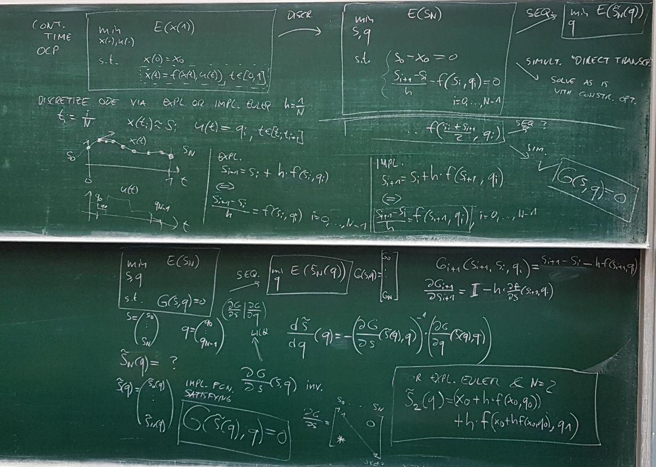
- Black board pictures
Project
You can find the project guidelines here, and the relevant dates in the following table. You can submit your ideas via email to florian.messerer@imtek.de
| until 25.06. | Initial idea submission (until 10am) |
| 25.06. | Project discussions in Q&A |
| 02.07. | Project discussions in exercise session |
| 09.07. | Project discussions in Q&A |
| 16.07. | Project discussions in exercise session |
| 23.07. | Project presentations |
| 06.08. | Project report deadline |
Matlab and CasADi installation
MATLAB is an environment for numerical computing based on a proprietary language that allows one to easily manipulate matrices and visualize data which will be very helpful in prototyping the algorithms presented during the lectures of this course. The University of Freiburg offers a free-of-cost license to students and staff which can be obtained following the instructions here. In order to be able to complete the exercises of this course, you will need a working installation of MATLAB. Follow the instructions at the provided link in order to install the software package.
CasADi is a symbolic framework for algorithmic differentiation and numerical optimization. In order to install CasADi, follow the instructions here. Download the binaries for your platform and, after having extracted them, add their location to MATLAB's path. To test your installation run the simple example described at the provided link. If successful, save the path by executing the command savepath. In this way, the location of the binaries will be known even after restarting MATLAB.